Unit 01 Data Science Project #

The final project for this unit will be a research project. Working with the data science tools we explored this unit, you are expected to tell a narrative story about a time in your life using data as evidence.

To be successful in this project, you should find a topic that is both interesting to you and answerable (at least in part) with data from your chosen dataset. Your teachers will help you make sure your project hypothesis achieves that.

👾 💬 Extra Examples

📖 Extra Examples HERE

[1] Timeline #

1️⃣ Plan your project and choose a research question.

2️⃣ Conduct the data analysis and create data visualizations.

3️⃣ Create a research poster to communicate your findings.

4️⃣ Present your findings to the class.

5️⃣ If interested, you may present your findings at Shuyuan Research Week in May. This is not required.

📅 You will have 6 in-class blocks to plan and complete the coding portion of this project.

[2] Starter Materials #

💻 You can find your project in your Google Drive: Project: Data Science.ipynb

✏️ For the poster, you may use Canva or any other service. It will be A3 size. You will begin the poster after you finish the coding portion.

[3] Assessment #

✅ The assessment is broken down into four criteria:

• Project Planning
• Data Analysis
• Data Visualization
• Data Communication

For each criteria you will be assigned a score from 0-3:

• 0 - no to no evidence of the concept
• 1 - limited evidence of the concept
• 2 - adequate evidence of the concept
• 3 - substantial evidence of the concept

[4] Success Claims #

💯 Successful computer scientists should be able to make the following claims:

• Project Planning
  • I can choose a relevant research question and determine appropriate forms of evidence
  • I can consistently track my progress with specific comments
• Data Analysis
  • I can prepare my dataset by adding and removing necessary columns or rows
  • I can combine and reorganize pieces of data to explore new relationships and support my research question
  • I can generate summary statistics (mean, median, mode, frequency count) for describing the data
  • I can write readable code by using descriptive names for modules, functions, and variables
  • I can write descriptive comments to describe complex pieces of the code
• Data Visualization
  • I can choose appropriate data visualizations to communicate my findings
  • I can display data visualizations that are thoughtfully sorted and easy to read
  • I can include appropriate title, axis, and labels for my visualizations
• Data Communication: Poster
  • I can explain the purpose and focus of the research
  • I can explain my methodology, including action steps and reasoning for restructuring the data
  • I can reflect on the meaning of the data and provide context of the results
  • I can discuss the limitations and potential biases of my data and analysis
  • I can consider potential future areas of investigation if I were to continue this project

Keep the success claims in mind when coding your project.

[5] Tips & Tricks #

Detecting Chinese Characters #

Here is an example of how to detect if there are Chinese characters in a string.

• You will need to import regex
• Then use regex.search() - it will return either True or False if there are Chinese characters

import regex

chinese_string = "上海 2025"

if regex.search(r'\p{Han}', chinese_string) == True:
  print("Has Chinese!")
else:
  print("No chinese")

Creating a New Column Based on Another Column #

📖 Here is a dataframe stored in the variable age_df. It stores names and ages.

📖 In one code block, you will write a function with your conditional statements. This function returns True or False, based on their age.

def get_if_adult(age):
    if age < 18:
        return False
    else:
        return True

📖 In another code block, you can apply the function to each value in a given row. Here it applies the function get_if_adult() to each row of the age columns, and stores the return value in a new column called is_adult.

# Apply the get_age_group function to the age column
age_df['is_adult']  = age_df.apply(lambda row: get_if_adult(row['age']), axis=1)

📖 Here is the updated dataframe.

This tutorial is based of this guide.

Find the top 1+ based on two columns #

For example, I want to find the top 1 show I watched each month.

📖 Here is a dataframe stored in the variable watch_history_df.

1️⃣ Count how many times we watched each show during each month. For this we must use groupby.

#this counts up how many times I watched each show in each month
top_show_df = watch_history_df.groupby(by=["month", "show"]).size().to_frame("count")

2️⃣ Next, sort the values. Sort by month, then the count. We use ascending for the month, since we want to start with the lowest number (1 for january). We use descending for count, since we want the most watched at the top.

#this sorts the new df first by month, then by the count
top_show_df = top_show_df.sort_values(['month', 'count'], ascending=[True, False])

3️⃣ Last, get the top 1 show for each month. To do this, we use groupby combined with head. If you want the top 3, you could use .head(3), etc.

#this gets the top 1 for every month
top_show_df = top_show_df.groupby('month').head(1)

📖 Here is the new dataframe top_show_df.

Find the mode of a column for each unique value in another column #

📖 Here is a dataframe stored in the variable age_df. It stores names, ages, is_adult, and house.

age_df.head()

📖 We want to see what is the mode of is_adult for each house. For this we must use groupby.

mode_isAdult_by_house_df =  age_df.groupby(['house'])['is_adult'].agg(pd.Series.mode).to_frame().reset_index()

📖 Here is the new dataframe mode_isAdult_by_house_df.

For metal, because True and False appear the same amount of times it returns both options.

mode_isAdult_by_house_df

This tutorial is based of this post.

Find the mean of a column for each unique value in another column #

📖 Here is a dataframe stored in the variable age_df. It stores names, ages, is_adult, and house.

age_df.head()

📖 We want to see what is the mean age for each value in is_adult. For this we must use groupby.

You could also replace .mean() with .max() or .min()

To round the mean, add .round(3) after .mean()

mean_isAdult_by_age_df =  df.groupby(['is_adult'])['age'].mean().to_frame().reset_index()

📖 Here is the new dataframe mean_isAdult_by_age_df.

mode_isAdult_by_house_df

Compare a value to the value right above it #

📖 Here is a dataframe stored in the variable watch_history_df. It stores shows, episodes, and genre.

watch_history_df.head()

📖 We want to add a column to see what the previous show was called. For this we must use shift.

You could also put a number in the brackets to shift more than just 1 row down

For example, .shift(2) or .shift(-1)

watch_history_df['previous'] = watch_history_df['show'].shift()
watch_history_df.head()

📖 Now we will add a new column to track if the show is the same as the previous one.

watch_history_df["repeat"] = watch_history_df["show"] == watch_history_df["previous"]
watch_history_df.head()

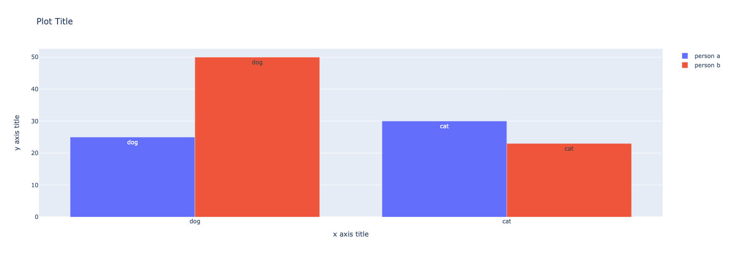
Grouped Bar Chart #

A grouped bar chart allows you to compare multiple sets of similar data.

📖 In this chart, we compare two people and their number of cats and dogs. Their data is stored in person1df and person2df. The dataframes are identical, except for the count column.

person1df         

person2df         

📖 This is how you create a group bar chart with two dataframes.

fig = go.Figure(data=[
    go.Bar(name='person a', x=person1df.animal, y=person1df.count, text=df1.Name),
    go.Bar(name='person b', x=person2df.animal, y=person2df.count, text=df2.Name)
])


fig.update_layout(
    barmode='group',
    title="Plot Title",
    xaxis_title="x axis title",
    yaxis_title="y axis title",
    )

fig.show()

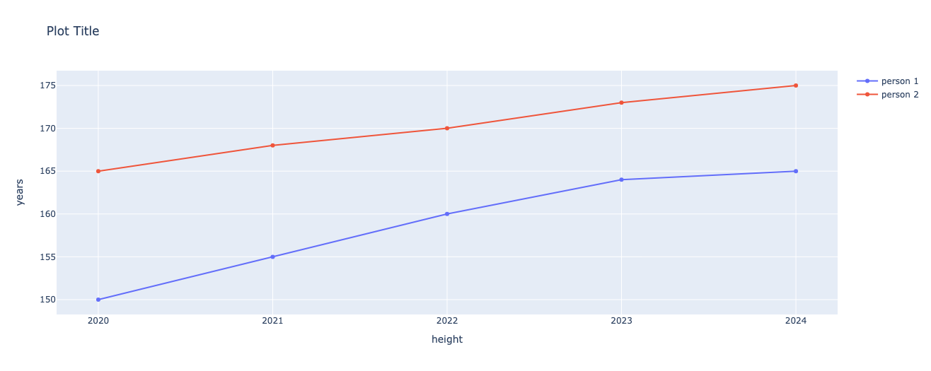
Line Charts with Many Lines #

A grouped bar chart allows you to compare multiple sets of similar data.

📖 In this chart, we compare two people and their heights over 5 years. Their data is stored in person1df and person2df. The dataframes are identical, except for the count column.

person1df         

person2df          

📖 This is how you create a group bar chart with two dataframes.

fig = go.Figure()

fig.add_trace(go.Scatter(x=person1df.year, y=person1df.height, name='person 1'))

fig.add_trace(go.Scatter(x=person2df.year, y=person2df.height, name='person 2'))

fig.update_xaxes(type='category') # only exisiting values for ticks 

fig.update_layout(
    title="Plot Title",
    xaxis_title="height",
    yaxis_title="years",
    )

fig.show()

Adding Other #

1️⃣ Make a new dataframe with just the top 5 artists For this we must use head.

# make a new df with just the top 5
top5_df = artist_totals.head(5)

2️⃣ Make a new dataframe with everyone except the top 5 artist. We use head again, but with a negative number.

# get everything except the top 5
other_df = artist_totals.tail(-5)

3️⃣ We add up the totals for all the other artists. To do this, we use sum.

#this gets the top 1 for every month
sum = other_df["total"].sum()

4️⃣ We add a new row for the other sum.

# create the new row
new_row = {'artist': 'Other', 'total': sum}
# make a new df that combines the top5_df with the new row
combo_df = top5_df.append(new_row, ignore_index = True)

📖 Here is the new dataframe combo_df.